Continuous learning

Documentation Index

Fetch the complete documentation index at: https://docs.deductive.ai/llms.txt

Use this file to discover all available pages before exploring further.

Most “AI for ops” products give you an answer and ask you to trust it. Deductive gives you the answer and the knowledge graph it pulled context from, plus the tree of decisions that produced the answer. You can read both, click into either, and reshape both. Together they form the continuous-learning loop: the knowledge graph keeps growing as you connect new sources; every investigation builds a decision tree; every comment reinforces or penalizes branches; the next investigation starts from a sharper baseline. This page is a tour of those two surfaces and how they learn.

​

Part 1. The knowledge graph

Open Agent → Knowledge in the left nav (or /knowledge). The Knowledge Archive is the index Deductive consults to ground every investigation, before it even forms a hypothesis. The graph has two pieces.

​

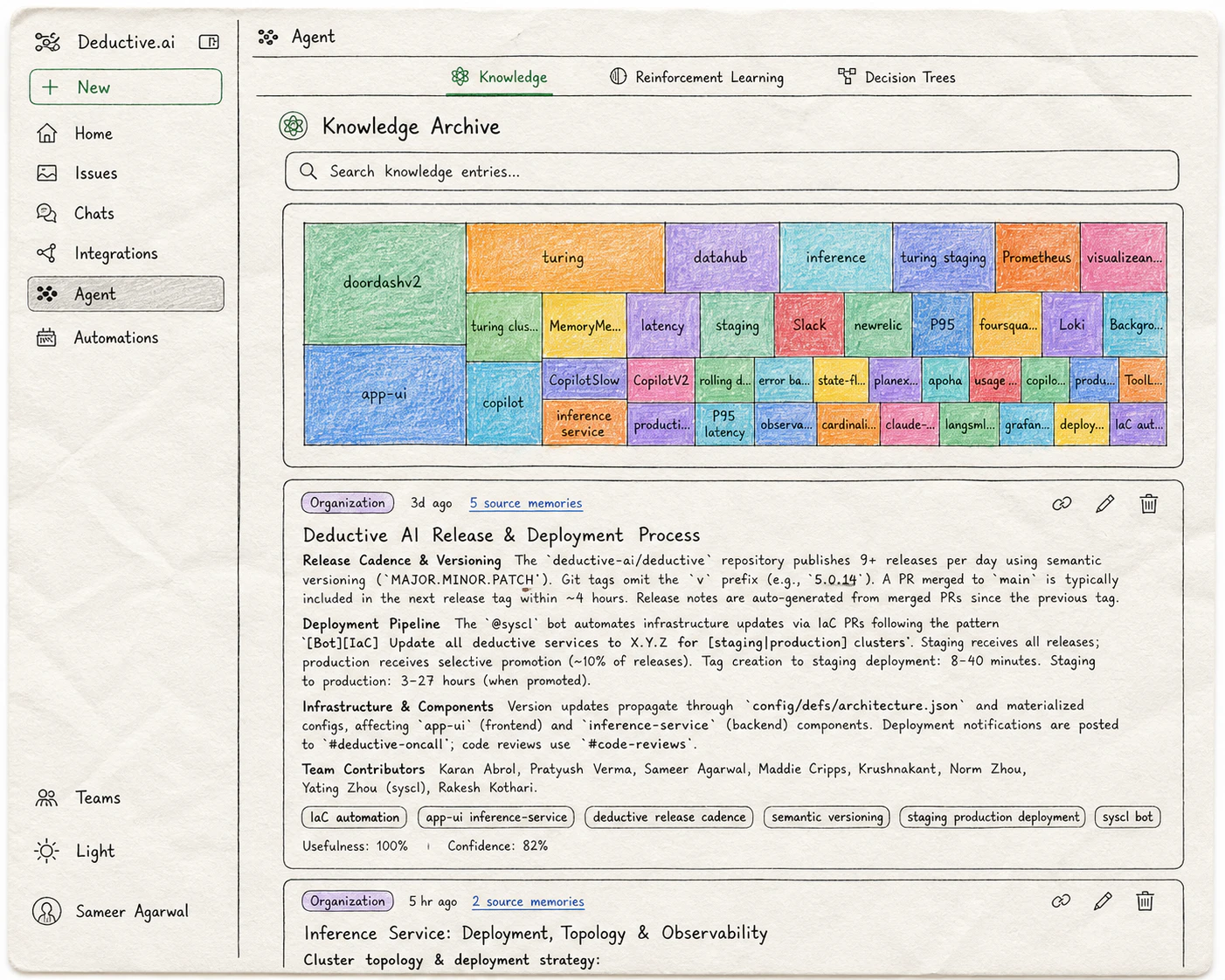
Knowledge entries

Short, curated pieces of context Deductive consults during investigations. Each entry has a title, a body, source memories it was built from, and a usefulness + confidence score. Examples of the kind of context an entry captures:

• “payments-api is owned by Team Atlas. Page Atlas via #oncall-atlas for prod issues.”
• “Anything in the legacy- namespace is being deprecated; don’t propose changes there.”
• “When redis_evictions spikes, look at cache-warmer deploy timing. They’re correlated 80% of the time.”
• “Our staging cluster routinely has error.rate=0.02 baseline; ignore unless it crosses 0.05.”

Click any entry to read its full body and the source memories it cites. You can rate an entry’s usefulness from the entry view, which feeds into the confidence score Deductive carries with it on future investigations.

​

The keyword graph

Beyond explicit entries, Deductive maintains a keyword-ranked graph across everything you’ve connected. Repos, dashboards, incidents, PRs. The treemap at the top of the Knowledge Archive visualizes the relative weight of each keyword across your stack: the bigger the tile, the more central that concept is to your team’s work. This isn’t just decoration. Deductive uses the graph to retrieve context at investigation time: when a question mentions checkout, the graph surfaces the repos, dashboards, recent incidents, and knowledge entries that historically co-occur with checkout. The denser and better-curated your graph, the sharper investigations get.

​

Part 2. Decision trees

Once a question is grounded in the knowledge graph, Deductive plans an investigation as a decision tree and executes it. The tree is the audit trail. Open Agent → Decision Trees in the left nav, then pick a monitor or symptom from the dropdown at the top of the page. Each selection loads the trees Deductive has built for that monitor over time.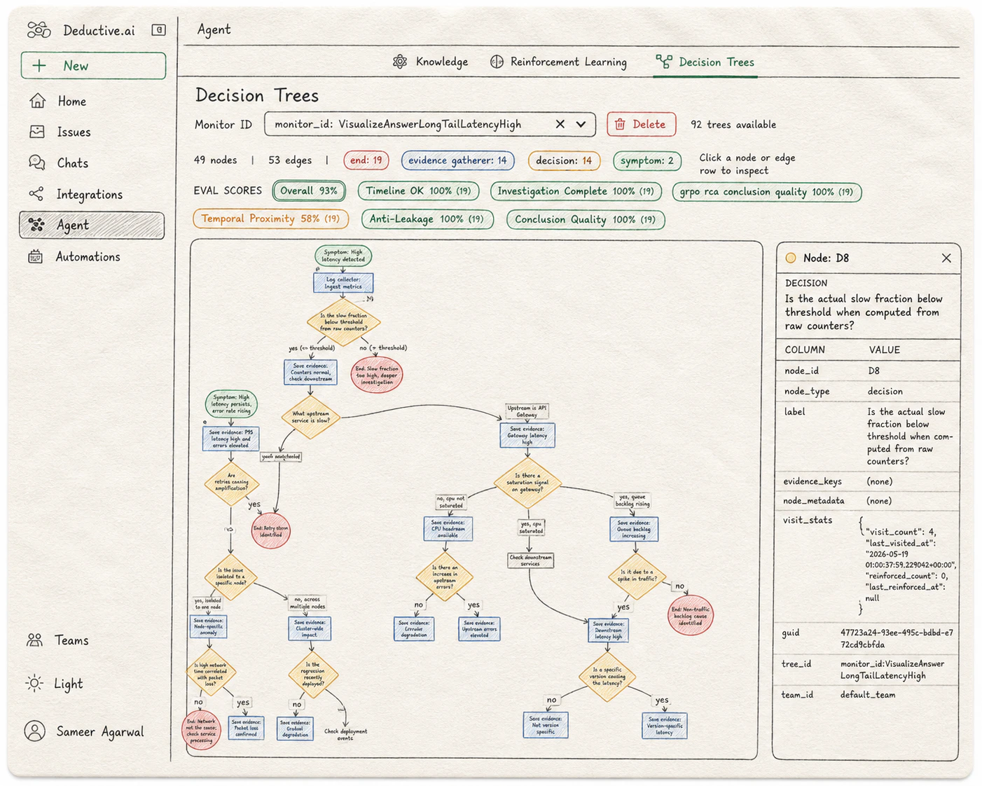

​

How to read it

Trees grow top-to-bottom. Each tree investigates a single monitor or symptom from the dropdown above. Above the tree, a header reports the counts: total nodes, total edges, and a breakdown by type (“end: 19 / evidence gatherer: 14 / decision: 14 / symptom: 2”). Edges carry the routing: a “yes” or “no” out of a decision diamond, or the outcome of an evidence gatherer that informed the next step.

​

Click into any node

Selecting a node opens a detail panel on the right with the node’s full metadata:

• node_id and node_type. The canonical id (e.g. D8) and category (symptom, decision, evidence_gatherer, end).
• label. The question the node is asking, or the evidence statement it captured.
• evidence_keys and node_metadata. Structured pointers to the data the node touched. Empty for purely-routing decision nodes; populated for evidence gatherers.
• visit_stats. How often this node has been traversed (visit_count), when it was last hit (last_visited_at), how many times it’s been reinforced as part of a canonical path (reinforced_count), and when (last_reinforced_at). This is the surface where reinforcement learning is visible at the node level.
• guid, tree_id, team_id. References for cross-linking and team scoping.

​

Eval scores

Above the tree, Deductive shows an eval scores row computed across the trees for the selected monitor. Each axis grades a different property of the reasoning. The number in parentheses is the sample size (how many trees were evaluated):

• Overall. The rollup across all axes.
• Timeline OK. Whether the events the tree references actually line up in time.
• Investigation Complete. Whether the tree explored enough branches before terminating.
• Temporal Proximity. Whether the evidence the tree cited was close enough in time to the symptom to be causally plausible.
• Anti-Leakage. Whether the tree avoided using information from after the symptom that wouldn’t have been available at investigation time.
• Conclusion Quality. How sharp and well-supported the terminal conclusions are.
• Domain-specific axes (e.g. grpo rca conclusion quality). Additional axes the evals team has trained for your stack.

A low score on any axis is the leading indicator of where to invest training. Drill into the trees that scored low on that axis, find the recurring failure mode, and reinforce a better path (see Teach Deductive).

​

How the graph and the tree work together

The knowledge graph is “what the agent always knows.” The decision tree is “what the agent did this time.” They’re two views of the same loop, and you can shape both.

​

Try this next